<home>
Jan /Feb 2020
Across the Bakken basin, oil productivity varies widely. A useful indicator is the area specific peak month performance of the wells – IP30. But, for the same acreage, IP30 has nearly doubled in the past 5 years as a result of improved completion techniques. To get a more absolute indication of land productivity, well performance has to be adjusted for these changes.
Productivity index map
To get a view of the geographic distribution of land productivity, the basin has been subdivided in squares of 3×3 miles and an IP30 quality index has been calculated for each square, based on the wells located in that square. The index is the average of the IP30 indexes of all the wells placed in that square since 2014. To take into account that average IP30 values have increased over time for the same acreage quality, as a result of improved completions, the IP30 index of each well has been calculated relative to the Bakken average IP30 of the year when the well’s IP30 happened. For example, in 2014, the Bakken IP30 average was 559 bopd. A well with IP30 of 700 bopd in that year was assigned an index of 700/559 = 1.23. In 2018, the Bakken IP30 average was around 1000 bopd. A well with an IP30 of 700 bopd in 2018 was assigned an index of 700/1000 = 0.7. That approach is certainly not perfect, but has been found to be a very useful way to get a measure of specific land productivity.
The result is shown in the map below. The map shows all the squares that have ever seen a horizontal well in North Dakota. The size of each square is 3×3 miles. The productivity differences are represented by different colours (blue= low to red= high). The relative Ip30 ranges associated with the different colours are shown in the summary table below.
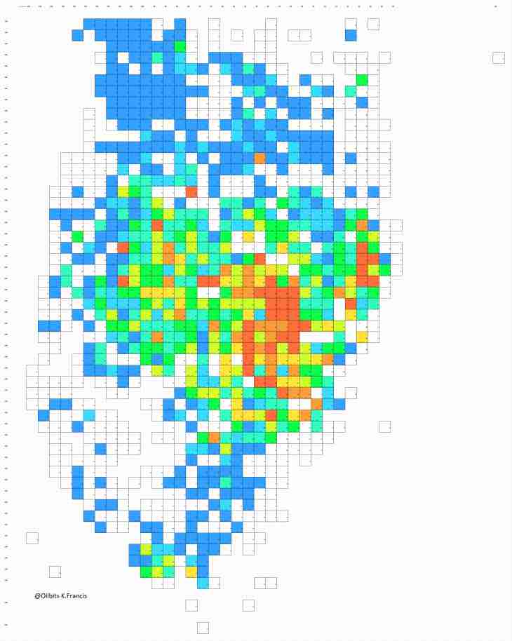
As the map shows, there is a core area (yellow to red colours) roughly comprising 20*40 sqm. Inside that area, the core of the core consists in an area of approx. 10*30 sqm. A second area to the right of roughly 20*20 sqm show average to slightly above average productivity. The red zone on the left side of the map largely represents EOG’s Parshall field. That field is now saturated with wells and the colour is the result of wells drilled there in 2014, when Parshall wells outperformed the Bakken average by 100%. Because of over-drilling, the few recent wells placed in the Parshall have underperformed the Bakken average by 25% to 30%.
Towards the periphery, the quality of the acreage diminishes. In the blue squares in the periphery, relatively few wells have been drilled. The uncoloured squares contain even less wells, all drilled before 2014, with very low relative IP30 values, requiring WTI prices around $150/bo to be of economic interest.
A dozen of such uncoloured squares can be found close to the core, surrounded by squares with average or better than average indexes, suggesting that these squares have potential. There may be reasons why these square have not been drilled after 2013. There are also a few square in the centre with no recorded well at all. These are usually areas under water. They contain horizontal wells drilled from the neighboring squares located on the shore.
Many squares have wells with legs extending into neighboring squares. If neighboring squares have different colors, a more precise representation would show a smooth color transition, but that doesn’t change the big picture. Because of the inter-dependencies between squares, the calculation of the saturation ratios of a single square may be misleading.
Remaining well inventory
Spacing and Saturation levels
The Bakken has 2 oil carrying benches of economic value: Middle Bakken (MB) and Three Forks (TF). Wells are typically placed in 1×2 miles Space units (SU).
To get an estimate of the remaining well inventory of the Basin, an assessment of the average number of wells per SU at the time of basin saturation in a few years has to be made. As has been described in the IP30 trend chapter, a few companies are now placing 12 wells in a space unit in two benches and occasionally even more. In earlier year, the number of wells in a space unit in was generally lower and conservative operators continue to place less than 12 wells in a SU.
It does normally not make sense to place additional wells in an existing SU, unless the SU contains only very few wells. If for example 5 equidistant wells (distance 1000 ft) have been drilled in a mile-wide section, adding a 6th well later would reduce the distance of that new well to neighboring wells to 500 ft – resulting in an uneconomic well.
As a result, at saturation point, the average number of Wells drilled in a space unit will be lower than the peak densities currently observed with certain operators.
Final density is also a function of land productivity. Economic logic dictates that the number of wells per SU declines with land productivity.
Based on observations and educated guesses, it has therefore been estimated that the average density per SU at saturation time in few years will be 10.8 wells per SU in the most productive SU, declining to 8 wells/SU in the SU’s with low productivity.
An example of final well density is provided by the Grail field. It’s a high-quality field largely owned by Qep, covering an area of roughly 70 sqm, consisting of approx. 35 SU. It’s now saturated with wells; the last completions having occurred in 2017. The Grail field seems to be one of the most densely drilled major areas in the Bakken. Earlier drilled SU’s show 7 wells per SU. A few SU, drilled in 2014 and 2015, contain up to 14 wells. Later, density was reduced again. But the average number of wells/SU of the field is “only” 9 wells. To conclude: the final well densities assumed here may be on the high side.
Quantitative Result
The total number of squares containing at least one well shown in the map amounts to 1124, covering a space of around 10,000 sqm. 423 uncoloured squares, usually located in the periphery, have not seen a well after 2013, usually because of very low well performance. It’s unlikely that new Wells will be drilled in these spaces unless WTI reaches a price range around $150/bo. Therefore, these spaces have been excluded from capacity calculations and only the coloured squares are considered for such calculations.
The coloured squares in the map comprise approx 6300 sqm. Squares with at least average productivity (green to red colours) amounts to 2100 sqm.
To take account of the fact that in some parts of the Basin only one bench is of economic interest, the number of squares has been adjusted for each productivity category for calculation purposes (column “adjusted squares”).
The column on the left side shows the average IP30 for each colour category as a % of the Bakken average. Wells in the blue coloured squares have an average IP30 of 51% of the IP30 of the average Bakken well.
The table below summarizes the results of the calculation of the remaining inventory for the different productivity categories (colours) for the Bakken basin. The Avg+ category includes all squares with at least average productivity (green color to red color) . The numbers for that category are shown in a separate line on the bottom of the table.

With the assumed average well densities at saturation time (column wells/ SU), the Avg+ inventory will be exhausted in approx 6 year, counted from the beginning of 2019, when assuming that the number of annual new wells in the Avg+ category remains at the 2018 level. Should the final number of wells / SU have been overestimated by one unit, Avg+ inventory exhaustion would occur one year earlier – at the end of 2023.
After Avg+ inventory exhaustion, only the below average productivity squares have inventory left. Drilling that inventory requires a significantly higher oil price and probably results in reduced drilling activity. In reality there will be no sudden cut off, but a gradual shift, as some operators will run out of quality inventory earlier than others.
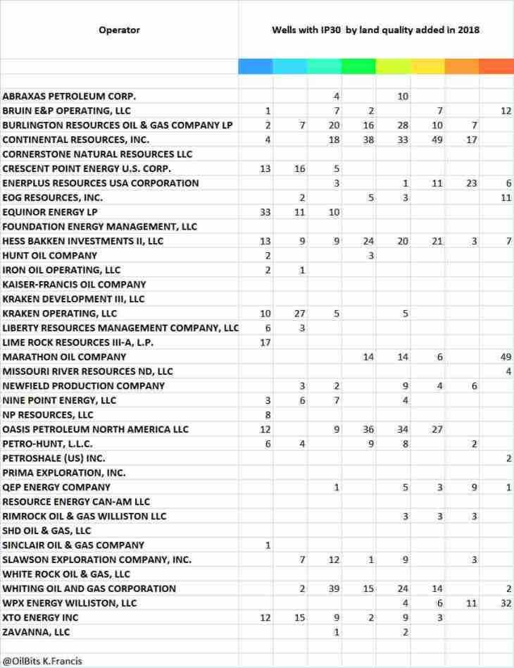
Operator specific data
The tables below show the results for each operator. Marginal operators with not more than 10 wells in the past 10 years are not shown.


The wells/SU numbers at saturation time used for each productivity category correspond to those used for the basin calculation. That’s obviously a simplification as different operators apply different spacing philosophies.
In the “Remaining Well Inventory” table, there are 2 columns on the right side. The first column shows the remaining number of Avg+ wells, the second column shows the years remaining until the Avg+ well inventory is exhausted, when drilling continues at the 2018 rate. For operators with a low number of 2018 wells (not more than 5 wells), no remaining year number is shown.
The remaining years are counted from the beginning of 2019.
As expected, QEP’s number of years left is on the low side, despite a reduced number of new wells in 2018. Among the large players, OAS’s and CLR’s remaining Avg+ inventory is also below average. 85% of CLR’s 2018 wells came from the Avg+ category – an extreme example of high grading.
XTO has by far the highest number of years of Avg+ inventory left. The company doesn’t have the largest inventory of such wells but, contrary to other operators, is barely consuming it. XTO had only 14 wells in the Avg+ category in 2018, but 36 in the below average categories.
